Python Programming

Why Deep Learning?

Deep Learning provides tools for learning complex non-linear models to deal with high-dimensional data (such as videos, text, audio files…).

The structure of deep learning models is such that its parameters can be trained in an efficient manner. By doing so, the deep learning models can capture and exploit the main features of the data under study.

What is Deep Learning?

Deep Learning techniques corresponds to the Machine Learning methods which rely on Artificial Neural Networks.

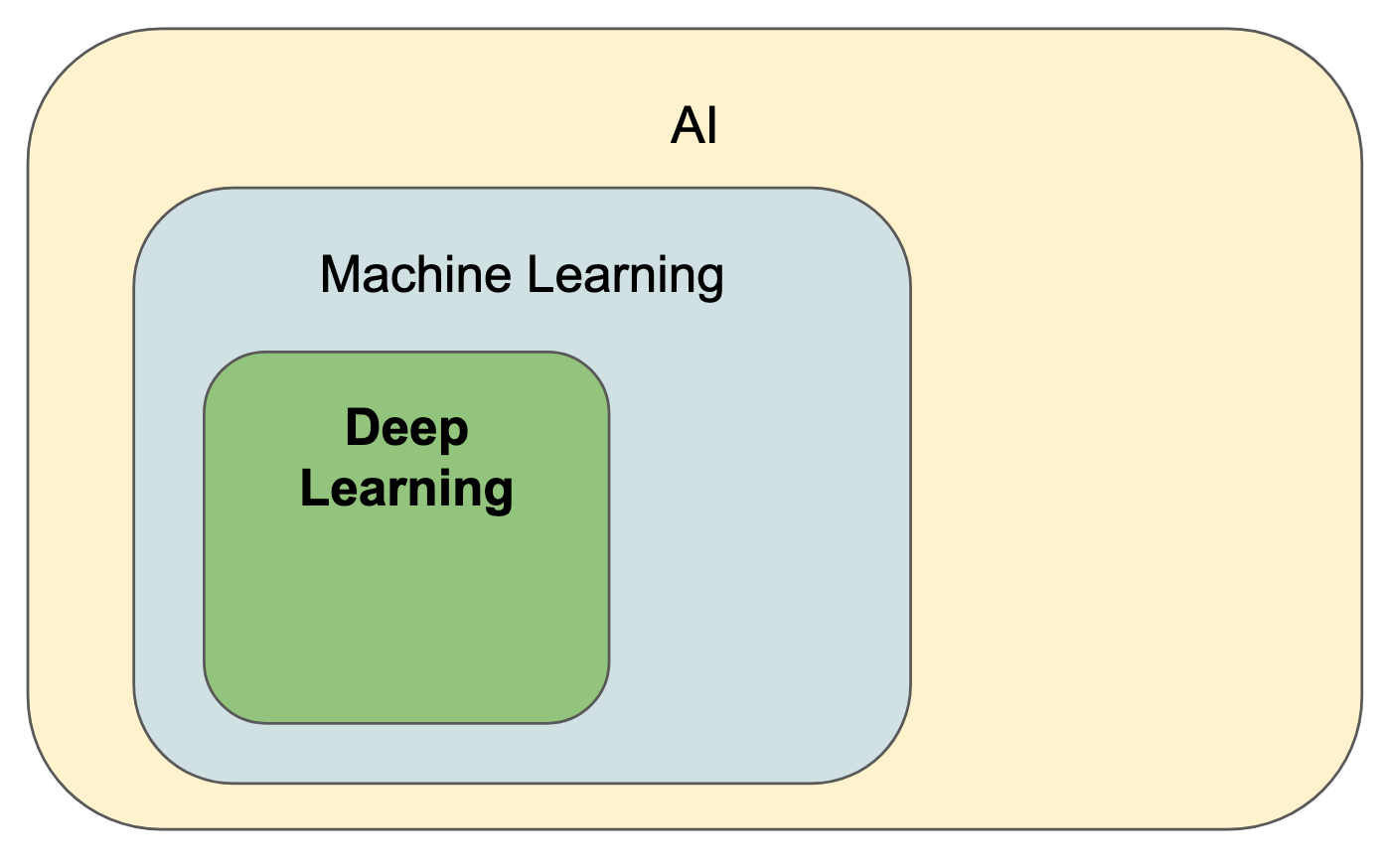
Artificial Neural Networks (ANN)

Generally, Artificial Neural Networks are graphs where:

• nodes represent the artificial neurons of the ANN. They all have an associated real number $b$ which influences its and an activation function $\phi : \mathbb{R}\rightarrow \mathbb{R}$. The activation function $\phi(\cdot)$ returns the output of the network. $\phi(\cdot)$ may not be linear.
• edges all have a weight $w$ ($w\in\mathbb{R}$). That weight $w$ quantifies the force of the transmitted signal between two neurons.

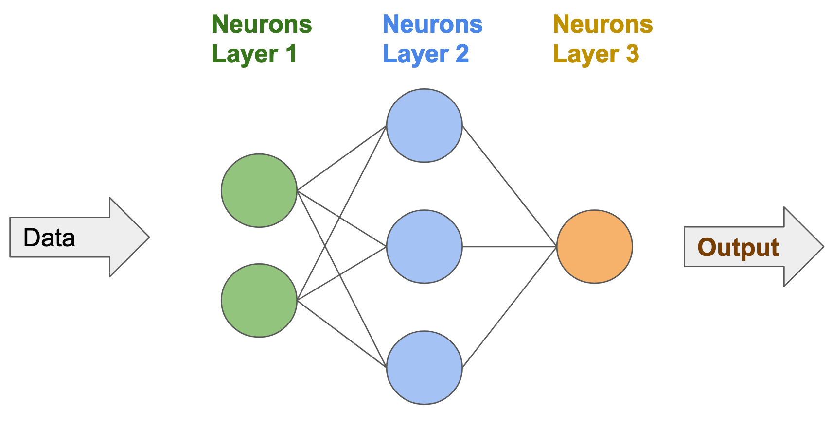
Suppose an input vector $\mathbf{x} = (x_1, x_2, \cdots, x_N)$ is fed to $N$ edges. All these edges share the same node. We write:

• $w_1, w_2, \cdots, w_N$ the respective weights of the edges.
• $b$ the bias of the neuron.
• $\phi$ the activation function of the neuron.

Then to compute the output of the neuron, we:

1. calculate the sum of the components from the input vector, weighted by the edges: $\sum_{i=1}^N x_i w_i$
2. add it to the bias $b$ of the neuron: $b + \sum_{i=1}^N x_i w_i$
3. compute the result of the activation function: $\phi(b + \sum_{i=1}^N x_i w_i)$

That result corresponds to the output of the artificial neuron.

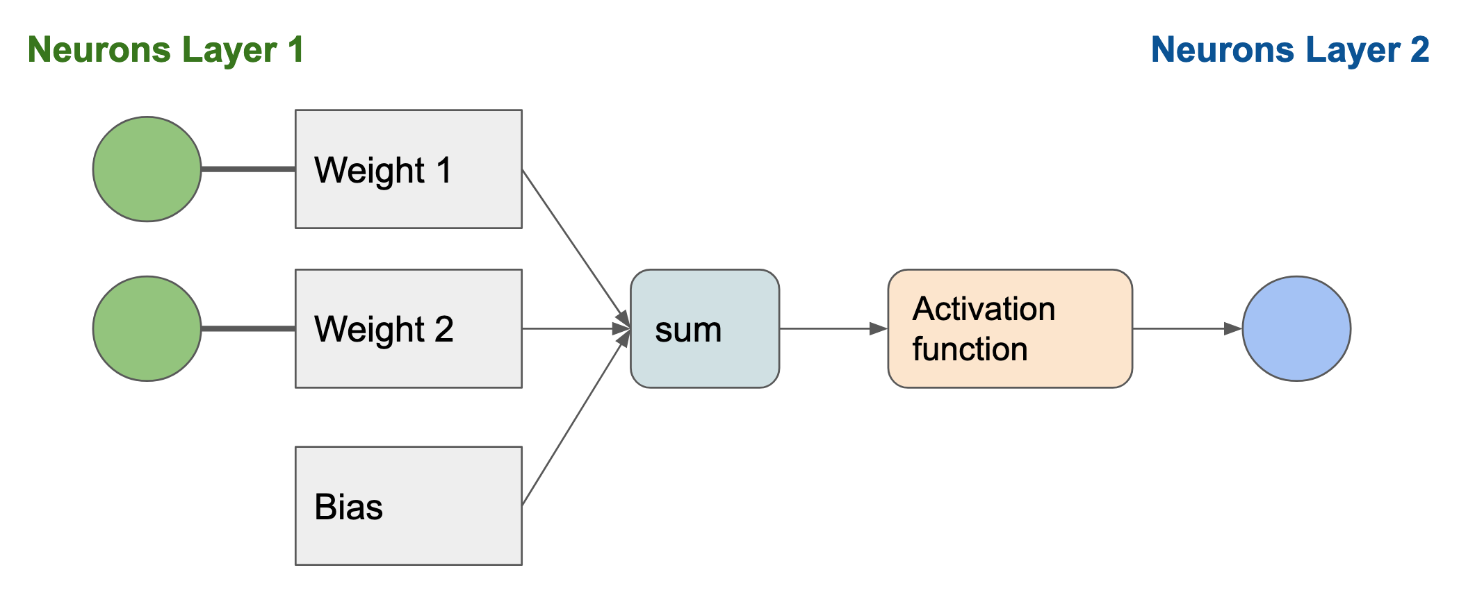
Artificial neurons can be combined to form different types of artificial neural networks (ANN). In rest of this chapter, we will focus on a simple type of ANN: the Multi-Layer Perceptron.

Multi-Layer Perceptrons (MLP)

In Multi-Layer Perceptrons, the neurons are grouped into layers. Each layer processes the output of its preceding layer, and transfers its result to the next layer.

An MLP is made of:

• the Input Layer, processing the input data
• $N_h$ Hidden Layers. The output of each hidden layer $h_i$ is calculated based on the output from the previous layer $h_{i-1}$.
• the Output Layers, computing the output of the neural network. That output will then be interpreted by the loss function $L(\cdot)$.

Also, in an MLP, two successive layers are always fully connected. In other words, all the neurons in the hidden layer $h_{i-1}$ are connected to all the neurons from the hidden layer $h_i$. Also, the same thing happens between the input layer and the first hidden layer $h_1$; and between the last hidden layer $h_{N_h}$ and the output layer.

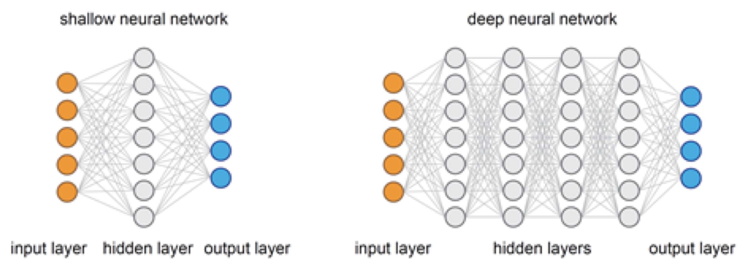
As the number of layers increases, the network gets deeper and:

• the network complexity increases
• the number of parameters increases
• more complicated functions can be modelled

For example, the image below shows two examples of MLPs. The MLP on the right has a larger depth than the one on the left.

Purpose

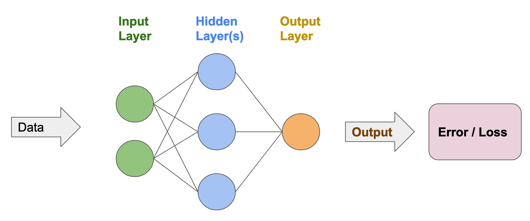
As explained before, the result obtained from the output layer is used to compute the loss function $L(\cdot)$. The goal is to find the edge weights $(w_e)_{e\in \text{edges}}$ and the neuronal biases $(b_n)_{n\in \text{neurons}}$ which minimise the loss function $L(\cdot)$.

How to optimise the parameters?

There are different ways to optimise the parameters of the neural network ($(w_e)_{e\in \text{edges}}$ and $(b_n)_{n\in \text{neurons}}$). Usually, the Deep Learning field uses first-order optimisation techniques. Those optimisation techniques rely on the estimation of the partial derivatives $\dfrac{\partial L}{\partial \cdot}$ with respect to the parameters of the neural network.

For example, the gradient descent algorithm is a first-order optimisation technique. It uses the partial derivatives of the loss function to update the parameters of the neural network: $w_e \leftarrow w_e - \lambda \dfrac{\partial L}{\partial w_e}\: \forall e\in\text{edges}$

$b_n \leftarrow b_n - \lambda \dfrac{\partial L}{\partial b_n}\: \forall n\in\text{neurons}$

(where $\lambda$ represents the learning rate of the gradient descent)

To compute the loss function partial derivatives $\dfrac{\partial L}{\partial \cdot}$, we usually use an algorithm called backpropagation.

We will not explain the backpropagation algorithm in detail in this course. These are covered in your Introduction to Machine Learning course. All you need to know is that the gradients are estimated by reversing the order of the neural network. The gradient of the loss function w.r.t the parameters at layer $i$ $\left(\dfrac{\partial L}{\partial w_e}\right)_{e\in \text{layer }h_{i}}$ is computed based on the gradient estimated from layer $i+1$: $\left(\dfrac{\partial L}{\partial w_e}\right)_{e\in \text{layer }h_{i+1}}$