Introduction to Deep Learning with PyTorch
Chapter 2: Gradient Descent
Gradient Descent: Illustration
Let’s illustrate the main principle of gradient descent in the case of a convex single-variable function:
More specifically, we consider the square function L : x \rightarrow x^2. In this case:
- \dfrac{\partial L}{\partial x} = 2x.
- L has a global minimum at x=0.
And the update rule is:
x \leftarrow x - \lambda \dfrac{\partial L}{\partial x}
Case when x > 0
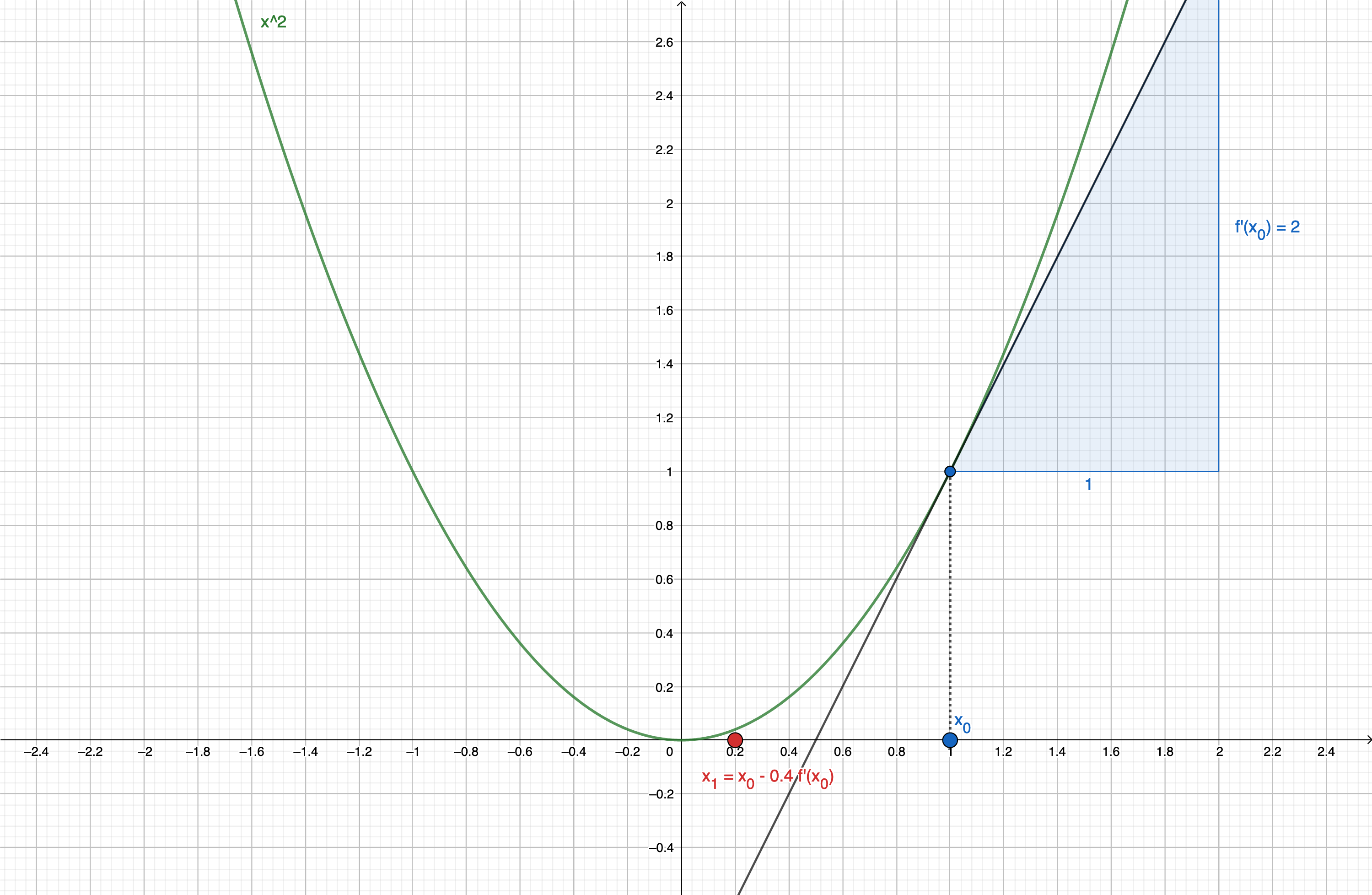
Let’s say we take x_0 = 1.
As x_0>0, \dfrac{\partial L}{\partial x}(x_0) > 0.
So, as x_1 \leftarrow x_0 - \lambda \dfrac{\partial L}{\partial x}(x_0):
- x_1 < x_0
- if \lambda is small enough, x_1 will be closer to 0. (see figure below, for \lambda=0.4 )

Case when x < 0
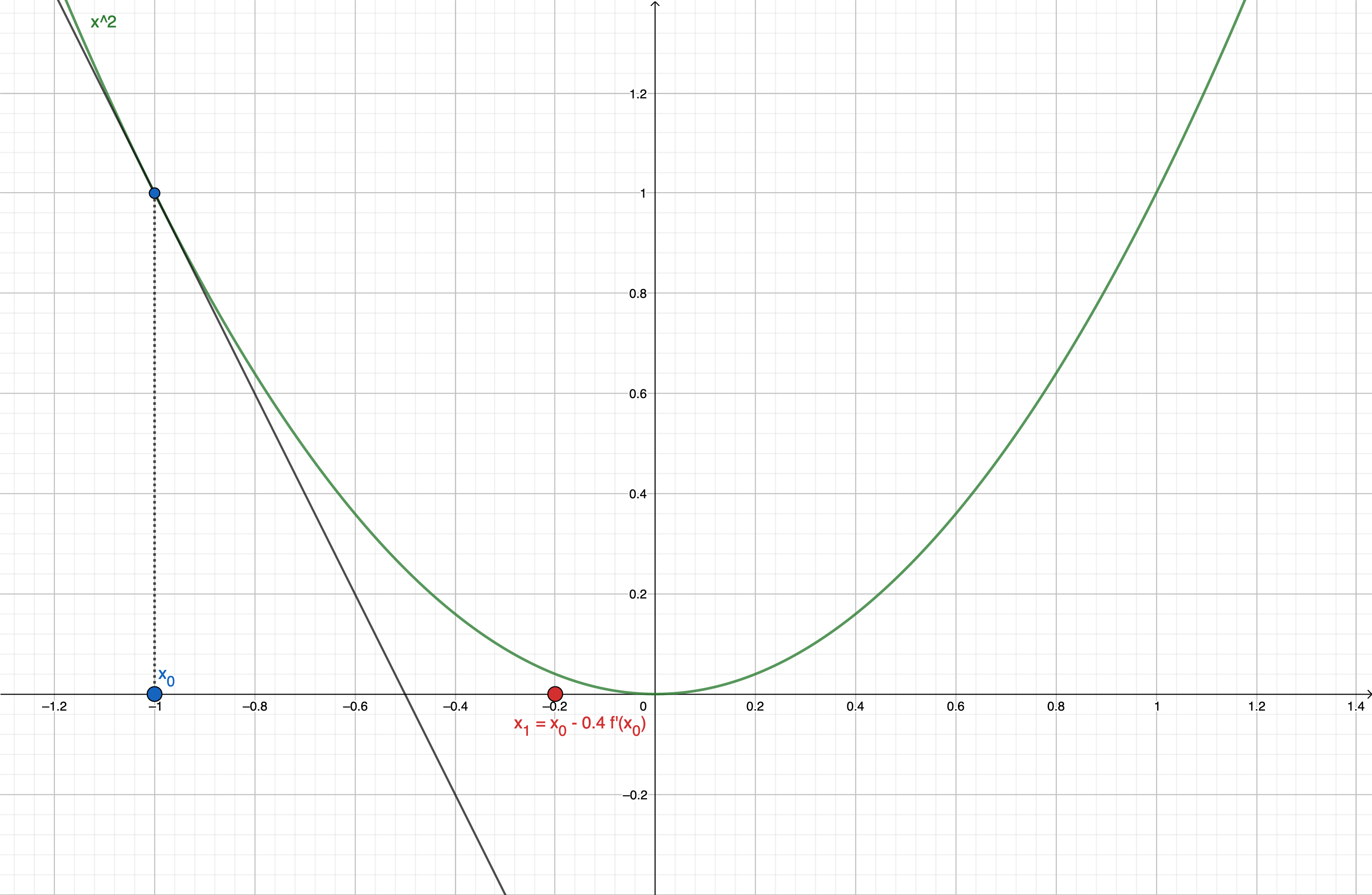
Let’s say we take x_0 = -1.
As x_0<0, \dfrac{\partial L}{\partial x}(x_0) < 0.
So, as x_1 \leftarrow x_0 - \lambda \dfrac{\partial L}{\partial x}(x_0):
- x_1 > x_0
- if \lambda is small enough, x_1 will be closer to 0. (see figure below, for \lambda=0.4 )

