Introduction to Deep Learning with PyTorch
Chapter 6: Introduction to Deep Learning
Deep Learning: In Practice - Example
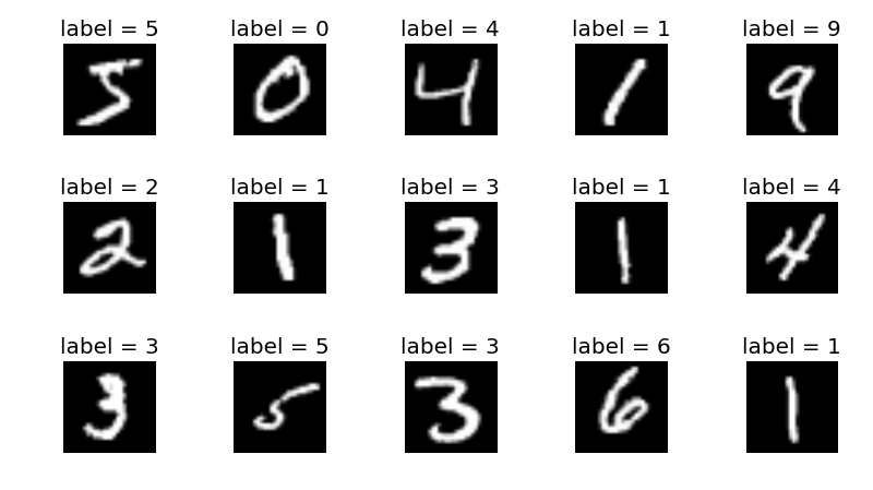
Consider we want to build a neural-network model \mathcal{M} for classifying black & white images of digits (from 0 to 9) from the MNIST dataset. Such a model can take as input an image of a digit, and output a prediction of that digit.

input
As input, our model needs to process batches of black and white images of size 28 \times 28. Such batches are tensors of shape: (N_{batch}, N_{channels}, W, H), where
- N_{batch} refers to the number of elements in the batch. It corresponds to the number of samples per gradient update.
- N_{channels} corresponds to the number of channels in the image. In the case of RGB color images, there are 3 channels: one for the red, one for the green and one for the blue. In our case, the images are black and white, so there is only one channel (for the intensity of the black color).
- W is the width of the image. In our case: W=28
- H is the height of the image. In our case: H=28
Thus, using MNIST images, our batches will have the following shape: (N_{batch}, 1, 28, 28).
In our case, we choose to flatten each image at the entry of our model so that it can be processed. Our batches then have the following shape: (N_{batch}, 1\times 28\times 28)
output and loss
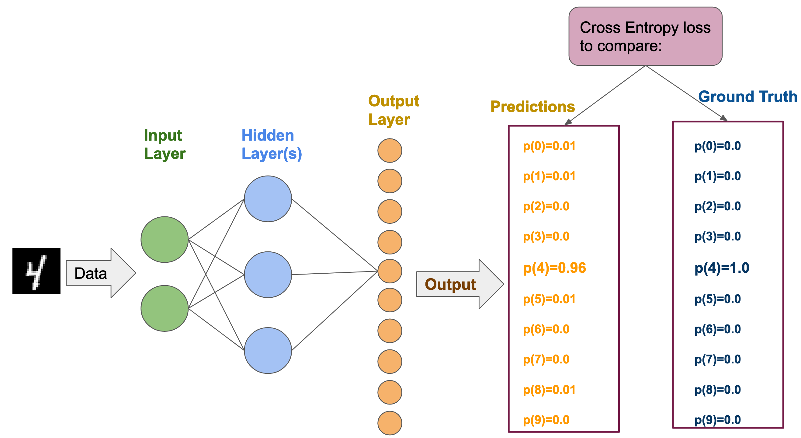
As an output, our model \mathcal{M} computes a vector of 10 values. Each one of these values is associated to a digit from 0 to 9.
Based on those output values, the cross-entropy loss estimates a vector of probabilities: [p(I=0), p(I=1), \cdots, p(I=9)]. where p(I=\alpha) refers to the probability that the image I has the label \alpha.
The cross-entropy loss estimates a distance between:
- the probabilities or predictions for each label: [p(I=0), p(I=1), \cdots, p(I=9)]
- and the ground truth label.
hidden structure
We will only consider a Multi-Layer Perceptron, with two fully-connected layers of size 64, between the input layer of size 1\times 28\times 28 and the output layer of size 10.
We equip each neuron in hidden layers with a ReLu activation function.
training and testing
Several optimisers (Adam, RMSProp, …) can be used. In our example, we will use Adam (the way it works is definitely beyond the scope of this lesson!).
And we choose to perform our training:
- with batches of size N_{batch}=32,
- for 5 epochs (each epoch is an iteration over the entire dataset).
The following section explains how to implement the model detailed above in practice!

